Constraint Handling
Evolutionary algorithms are usually unconstrained optimization procedures. In this tutorial, we present several ways of adding different types of constraints to your evolutions. This tutorial is based on the paper by Coello Coello [CoelloCoello2002].
Penalty Function
Penalty functions are the most basic way of handling constrains for individuals that cannot be evaluated or are forbidden for problem specific reasons, when falling in a given region. The penalty function gives a fitness disadvantage to these individuals based on the amount of constraint violation in the solution. For example, instead of evaluating an individual violating a constraint, one can assign a desired value to its fitness. The assigned value can be constant or increasing (decreasing for maximization) as the distance to a valid solution increases. The following figure shows the fitness function \(g(x)\) (in green) and the penalty function \(h(x)\) (in red) of a one attribute individual, subject to the constraint \(3 < x < 7\). The continuous line represent the fitness that is actually assigned to the individual \(f(x) = \left\lbrace \begin{array}{cl}g(x) &\mathrm{if}~3 < x < 7\\h(x)&\mathrm{otherwise}\end{array} \right.\).
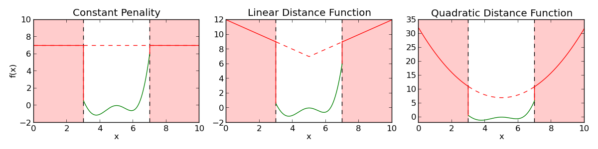
The figure on the left uses a constant offset \(h(x) = \Delta\) when a constraint is not respected. The center plot uses the euclidean distance in addition to the offset to create a bowl like fitness function \(h(x) = \Delta + \sqrt{(x-x_0)^2}\). Finally, the right plot uses a quadratic distance function to increase the attraction of the bowl \(h(x) = \Delta + (x-x_0)^2\), where \(x_0\) is the approximate center of the valid zone.
In DEAP, a penalty function can be added to any evaluation function using the
DeltaPenalty decorator provided in the tools
module.
from math import sin
from deap import base
from deap import tools

def evalFct(individual):
    """Evaluation function for the individual."""
    x = individual[0]
    return (x - 5)**2 * sin(x) * (x/3),

def feasible(individual):
    """Feasibility function for the individual. Returns True if feasible False
    otherwise."""
    if 3 < individual[0] < 7:
        return True
    return False

def distance(individual):
    """A distance function to the feasibility region."""
    return (individual[0] - 5.0)**2

toolbox = base.Toolbox()
toolbox.register("evaluate", evalFct)
toolbox.decorate("evaluate", tools.DeltaPenalty(feasible, 7.0, distance))
The penalty decorator takes 2 mandatory arguments and an optional one. The first argument is a function returning the validity of an individual according to user defined constraints. The second argument is a constant value (\(\Delta\)) returned when an individual is not valid. The optional argument is a distance function between an invalid individual and the valid region. This last argument takes on the default value of 0. The last example shows how the right plot of the top image was obtained.
References
Coelle Coello, C. A. Theoretical and numerical constraint-handling techniques used with evolutionary algorithms: a survey of the state of the art. Computer Methods in Applied Mechanics and Engineering 191, 1245–1287, 2002.